Denoising ADT

In this tutorial, we go through steps for ADT denoising in CITE-seq.

We will use the 10xPBMC5k CITE-seq dataset, which contained about five thousands cells stained with a panel of 32 antibodies. The original dataset was downloaded from 10x genomics dataset, and the processed and annotation data is available at scAR-reproducibility/data

Note

To run this notebook on your device, you need to install .

Alternatively, you can also run this notebook on Colab

# Run this cell to install scar in Colab
# Skip this cell if running on your own device

%pip install scanpy
%pip install git+https://github.com/Novartis/scAR.git
%pip install matplotlib==3.1.3  # Specify this matplotlib version to avoid errors

import numpy as np
import pandas as pd
import matplotlib.pyplot as plt
import seaborn as sns
import scanpy as sc
from scar import model

import warnings
warnings.simplefilter("ignore")

Matplotlib is building the font cache; this may take a moment.

Load data

Cells were annotated using well-established markers, see the scAR manuscript for details. For the tutoring purpose, the processed file (CITEseq_PBMCs_5k.h5ad) is provided.

!git clone https://github.com/CaibinSh/scAR-reproducibility.git

PBMCs5k = sc.read('scAR-reproducibility/data/CITEseq_PBMCs_5k.h5ad')

fatal: destination path 'scAR-reproducibility' already exists and is not an empty directory.

visualization of cell types

sc.settings.set_figure_params(dpi=150,figsize = (3, 3.1))

sc.pl.umap(PBMCs5k, size=10, color=["subtype"],color_map="viridis",legend_loc="on data", frameon=False, legend_fontsize=5)

Raw count matrix

Get a dataframe of ADT raw count as the input of scar

raw_ADT = PBMCs5k[:, PBMCs5k.var_names.str.endswith('_TotalSeqB')].to_df()

raw_ADT.columns = raw_ADT.columns.str.replace('_TotalSeqB','')

raw_ADT.head()

	CD3	CD4	CD8a	CD11b	CD14	CD15	CD16	CD19	CD20	CD25	...	CD197	CD274	CD278	CD335	PD-1	HLA-DR	TIGIT	IgG1_control	IgG2a_control	IgG2b_control
CCGGGTAGTTCAAACC-1	876.0	968.0	8.0	10.0	8.0	9.0	1.0	3.0	10.0	3.0	...	20.0	2.0	29.0	6.0	6.0	14.0	4.0	3.0	3.0	2.0
CTTTCGGTCCGCAACG-1	516.0	664.0	4.0	4.0	4.0	6.0	0.0	3.0	1.0	2.0	...	15.0	1.0	26.0	5.0	5.0	8.0	1.0	1.0	3.0	0.0
TCTACCGGTGTAAACA-1	666.0	837.0	5.0	10.0	6.0	5.0	1.0	4.0	7.0	4.0	...	30.0	1.0	36.0	2.0	5.0	9.0	1.0	3.0	3.0	2.0
ATAGACCCATAATGCC-1	352.0	709.0	3.0	7.0	8.0	12.0	3.0	4.0	4.0	2.0	...	13.0	2.0	100.0	6.0	12.0	9.0	4.0	2.0	2.0	2.0
TCTATACAGGGTATAT-1	289.0	861.0	7.0	3.0	8.0	4.0	2.0	4.0	9.0	21.0	...	10.0	3.0	31.0	3.0	3.0	11.0	1.0	4.0	4.0	4.0

5 rows × 32 columns

Ambient profile

Get a dataframe of ADT ambient profile as the input of scar

ambient_profile = PBMCs5k.uns['ambient_profile']

ambient_profile.head()

	ambient_profile
CD3	0.049876
CD4	0.048823
CD8a	0.023453
CD11b	0.083170
CD14	0.107178

IMPORTANT

In ‘CITEseq’ mode, we do not recommend running scar using default setting (i.e. estimating ambient profile by averaging cells). Instead, we recommend calculating ambient profile by averaging cell-free droplets. Calculation of ambient profile is key to precise denoising.

See an example for calculating ambient profile.

Training

ADT_scar = model(raw_count = raw_ADT,
                 ambient_profile = ambient_profile,  # Providing ambient profile is recommended for CITEseq; in other modes, you can leave this argument as the default value -- None
                 feature_type = 'ADT', # "ADT" or "ADTs" for denoising protein counts in CITE-seq
                 count_model = 'binomial',   # Depending on your data's sparsity, you can choose between 'binomial', 'possion', and 'zeroinflatedpossion'
                )

ADT_scar.train(epochs=500,
               batch_size=64,
               verbose=True
              )

# After training, we can infer the true protein signal
ADT_scar.inference()  # by defaut, batch_size=None, set a batch_size if getting GPU memory issue

2023-05-01 16:29:45|INFO|model|No GPU detected. Use CPU instead.
2023-05-01 16:29:47|INFO|VAE|Running VAE using the following param set:
2023-05-01 16:29:47|INFO|VAE|...denoised count type: ADT
2023-05-01 16:29:47|INFO|VAE|...count model: binomial
2023-05-01 16:29:47|INFO|VAE|...num_input_feature: 32
2023-05-01 16:29:47|INFO|VAE|...NN_layer1: 150
2023-05-01 16:29:47|INFO|VAE|...NN_layer2: 100
2023-05-01 16:29:47|INFO|VAE|...latent_space: 15
2023-05-01 16:29:47|INFO|VAE|...dropout_prob: 0.00
2023-05-01 16:29:47|INFO|VAE|...expected data sparsity: 0.90
2023-05-01 16:29:47|INFO|model|kld_weight: 1.00e-05
2023-05-01 16:29:47|INFO|model|learning rate: 1.00e-03
2023-05-01 16:29:47|INFO|model|lr_step_size: 5
2023-05-01 16:29:47|INFO|model|lr_gamma: 0.97

Training: 100%|██████████| 500/500 [02:52<00:00,  2.90it/s, Loss=1.0789e+02]

The denoised counts are saved in ADT_scar.native_counts and can be used for downstream analysis.

denoised_ADT = pd.DataFrame(ADT_scar.native_counts, index=raw_ADT.index, columns=raw_ADT.columns)

denoised_ADT.head()

	CD3	CD4	CD8a	CD11b	CD14	CD15	CD16	CD19	CD20	CD25	...	CD197	CD274	CD278	CD335	PD-1	HLA-DR	TIGIT	IgG1_control	IgG2a_control	IgG2b_control
CCGGGTAGTTCAAACC-1	865.0	973.0	0.0	0.0	0.0	5.0	0.0	0.0	0.0	0.0	...	9.0	0.0	26.0	0.0	6.0	0.0	0.0	0.0	0.0	0.0
CTTTCGGTCCGCAACG-1	502.0	648.0	0.0	0.0	0.0	3.0	0.0	0.0	0.0	0.0	...	7.0	0.0	23.0	0.0	1.0	0.0	0.0	0.0	0.0	0.0
TCTACCGGTGTAAACA-1	660.0	855.0	0.0	0.0	0.0	3.0	0.0	0.0	2.0	0.0	...	9.0	0.0	34.0	0.0	4.0	0.0	0.0	0.0	0.0	0.0
ATAGACCCATAATGCC-1	362.0	706.0	0.0	0.0	0.0	3.0	0.0	0.0	0.0	1.0	...	5.0	0.0	97.0	0.0	4.0	0.0	0.0	0.0	0.0	0.0
TCTATACAGGGTATAT-1	292.0	870.0	0.0	0.0	0.0	4.0	0.0	0.0	1.0	21.0	...	6.0	0.0	26.0	0.0	0.0	0.0	0.0	0.0	0.0	0.0

5 rows × 32 columns

Visualization

Plot setting

from matplotlib import pylab

params = {'legend.fontsize': 6,
          'legend.title_fontsize': 8,
          'figure.facecolor':"w",
          'figure.figsize': (6, 4.5),
         'axes.labelsize': 6,
         'axes.titlesize':8,
         'axes.linewidth': 0.5,
         'xtick.labelsize':6,
         'ytick.labelsize':6,
         'axes.grid':False,}
pylab.rc('font',**{'family':'serif','serif':['Palatino'],'size':10})
pylab.rcParams.update(params);

sns.set_palette("muted");
sns.set_style("ticks");
sns.despine(offset=4, trim=True);

<Figure size 900x675 with 0 Axes>

Boxplot of ADT counts per cell type

Prepare a dataframe for visualization

denoised_ADT_stacked = np.log2(denoised_ADT+1).stack().to_frame('log2(ADT+1)').rename_axis(['cells', 'ADTs']).reset_index().set_index('cells')
denoised_ADT_stacked = denoised_ADT_stacked.join(PBMCs5k.obs)
denoised_ADT_stacked['count'] = 'scar-denoised ADT'

raw_ADT_stacked = np.log2(raw_ADT+1).stack().to_frame('log2(ADT+1)').rename_axis(['cells', 'ADTs']).reset_index().set_index('cells')   # log scale for visualization,
raw_ADT_stacked = raw_ADT_stacked.join(PBMCs5k.obs) # Add cell type information
raw_ADT_stacked['count'] = 'raw ADT'

ADTs_stacked = raw_ADT_stacked.append(denoised_ADT_stacked)

ADTs_stacked.head()

	ADTs	log2(ADT+1)	celltype	subtype	count
AAACCCAAGAGACAAG-1	CD3	4.700440	Monocytes	intermediate mono	raw ADT
AAACCCAAGAGACAAG-1	CD4	7.366322	Monocytes	intermediate mono	raw ADT
AAACCCAAGAGACAAG-1	CD8a	4.087463	Monocytes	intermediate mono	raw ADT
AAACCCAAGAGACAAG-1	CD11b	11.556027	Monocytes	intermediate mono	raw ADT
AAACCCAAGAGACAAG-1	CD14	9.445015	Monocytes	intermediate mono	raw ADT

Boxplot visualization of ADT counts per cell type before and after denoising.

marker = "CD19"
tmp = ADTs_stacked[ADTs_stacked['ADTs']==marker]
plt.figure(figsize=(3, 1.8))

g = sns.boxplot(x="subtype",
                y="log2(ADT+1)",
                data=tmp,
                hue="count",
                hue_order=['raw ADT', 'scar-denoised ADT'],
                orient="v",
                dodge=True,
                width=0.8,
                showfliers=False,
                linewidth=0.5,
           );

g.legend_.set_title('')
g.set(xlabel='',title=f'{marker} protein counts');
g.set_xticklabels(g.get_xticklabels(),rotation=45, ha='right');

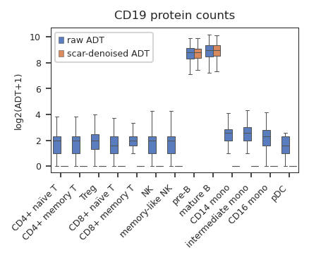
CD19 is a B cell specific marker, raw CD19 counts are detected in every cell type, while denoised counts are only observed in B cells.

Similarly, we observed ambient ADTs of other markers and scar can remove these ambient signals but preserve ‘true’ ADTs.

for marker in ["CD3", "CD4", "CD8a", "CD11b", "PD-1", "IgG2a_control"]:
    tmp = ADTs_stacked[ADTs_stacked['ADTs']==marker]
    plt.figure(figsize=(3, 1.8))
    g = sns.boxplot(x="subtype",
                    y="log2(ADT+1)",
                    data=tmp,
                    hue="count",
                    hue_order=['raw ADT', 'scar-denoised ADT'],
                    orient="v",
                    dodge=True,
                    width=0.8,
                    showfliers=False,
                    linewidth=0.5,
               );
    g.legend_.set_title('')
    g.set(xlabel='', title=f'{marker} protein counts');
    g.set_xticklabels(g.get_xticklabels(),rotation=45, ha='right')

UMAP of ADT and RNA

match ADT name and transcript name

prot2gene = PBMCs5k.uns['prot2gene']

Expression of mRNA

mRNA = PBMCs5k[:, list(prot2gene.values())].to_df()
mRNA.columns = mRNA.columns.astype(str)+'_RNA'

raw_ADT.columns = 'raw_' + raw_ADT.columns.astype(str)
denoised_ADT.columns = 'denoised_' + denoised_ADT.columns.astype(str)
PBMCs5k.obs = PBMCs5k.obs.join(mRNA).join(raw_ADT).join(denoised_ADT)

sc.settings.set_figure_params(dpi = 150, figsize = (1.5, 1.5), fontsize = 6)

for marker in ["CD3", "CD4", "CD8a", "CD19", "CD11b", "PD-1"]:
    raw_prot_label = f'raw_{marker}'
    denoised_prot_label = f'denoised_{marker}'
    RNA_label = f'{prot2gene[marker]}_RNA'
    sc.pl.umap(PBMCs5k,
               size = 5,
               color = [raw_prot_label, denoised_prot_label, RNA_label],
               color_map = "viridis",
               frameon = False,
               vmax = [8, 8, 3],
               vmin = 0,
               wspace = 0.1
              )