Denoising scATACseq#
In this tutorial, we will walk through the steps for denoising peak counts in species-mixing scATACseq data.
In this experiment, an equal number of human GM12878 nuclei and mouse EL4 nuclei were pooled and sequenced, ATAC signals from the other organism were unambiguously ambient contamination. The original dataset is downloaded from 10x genomics dataset.
Note
To run this notebook on your device, you need to install .
Alternatively, you can also run this notebook on Colab ![]()
[ ]:
# Run this cell to install scar in Colab
# Skip this cell if running on your own device

%pip install scanpy
%pip install git+https://github.com/Novartis/scAR.git
%pip install matplotlib==3.1.3  # Specify this matplotlib version to avoid errors
[1]:
import numpy as np
import pandas as pd
import matplotlib.pyplot as plt
import seaborn as sns
import scanpy as sc
from scar import model, setup_anndata

import warnings
warnings.simplefilter("ignore")
Download data#
The raw and filtered count matrices can be downloaded from 10x Dataset.
The raw data#
cellranger output: raw_peak_bc_matrix
[2]:
hgmm10k_scATACseq_raw = sc.read_10x_h5(filename='10k_hgmm_ATACv2_nextgem_Chromium_Controller_raw_peak_bc_matrix.h5',
                                       backup_url='https://cf.10xgenomics.com/samples/cell-atac/2.1.0/10k_hgmm_ATACv2_nextgem_Chromium_Controller/10k_hgmm_ATACv2_nextgem_Chromium_Controller_raw_peak_bc_matrix.h5',
                                      gex_only=False);
hgmm10k_scATACseq_raw.var_names_make_unique();
The filtered data#
cellranger output: filtered_peak_bc_matrix
[3]:
hgmm10k_scATACseq = sc.read_10x_h5(filename='10k_hgmm_ATACv2_nextgem_Chromium_Controller_filtered_peak_bc_matrix.h5',
                                   backup_url='https://cf.10xgenomics.com/samples/cell-atac/2.1.0/10k_hgmm_ATACv2_nextgem_Chromium_Controller/10k_hgmm_ATACv2_nextgem_Chromium_Controller_filtered_peak_bc_matrix.h5',
                                   gex_only=False);
hgmm10k_scATACseq.var_names_make_unique();
[4]:
sc.pp.calculate_qc_metrics(hgmm10k_scATACseq, inplace=True)
[5]:
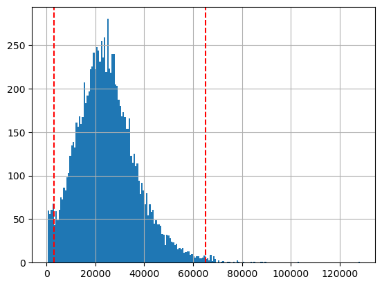
hgmm10k_scATACseq.obs['total_counts'].hist(bins=200);
plt.axvline(3000, c='r', ls='--')
plt.axvline(65000, c='r', ls='--')
[5]:
<matplotlib.lines.Line2D at 0x7f1847ba7fe0>
[6]:
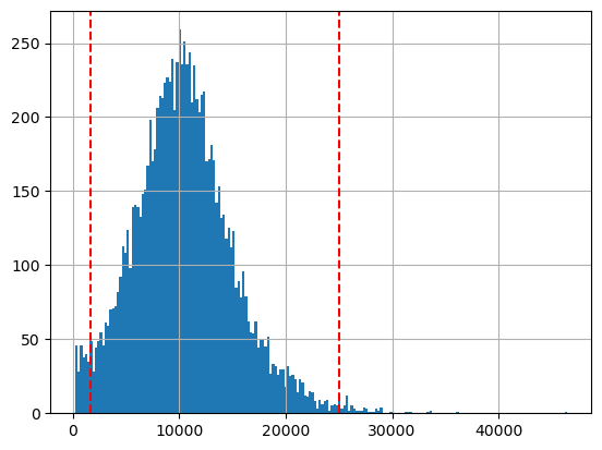
hgmm10k_scATACseq.obs['n_genes_by_counts'].hist(bins=200);
plt.axvline(1700, c='r', ls='--')
plt.axvline(25000, c='r', ls='--')
[6]:
<matplotlib.lines.Line2D at 0x7f1847bfe480>
[7]:
hgmm10k_scATACseq.var.head()
[7]:
| gene_ids | feature_types | derivation | genome | n_cells_by_counts | mean_counts | log1p_mean_counts | pct_dropout_by_counts | total_counts | log1p_total_counts | |
|---|---|---|---|---|---|---|---|---|---|---|
| GRCh38_chr1:181026-181833 | GRCh38_chr1:181026-181833 | Peaks | GRCh38 | 84 | 0.014667 | 0.014561 | 99.215247 | 157.0 | 5.062595 | |
| GRCh38_chr1:267559-268474 | GRCh38_chr1:267559-268474 | Peaks | GRCh38 | 78 | 0.014481 | 0.014377 | 99.271300 | 155.0 | 5.049856 | |
| GRCh38_chr1:585752-586649 | GRCh38_chr1:585752-586649 | Peaks | GRCh38 | 62 | 0.011584 | 0.011518 | 99.420777 | 124.0 | 4.828314 | |
| GRCh38_chr1:605062-605946 | GRCh38_chr1:605062-605946 | Peaks | GRCh38 | 45 | 0.008315 | 0.008280 | 99.579596 | 89.0 | 4.499810 | |
| GRCh38_chr1:627577-628437 | GRCh38_chr1:627577-628437 | Peaks | GRCh38 | 26 | 0.004858 | 0.004846 | 99.757100 | 52.0 | 3.970292 |
[8]:
hgmm10k_scATACseq.var['n_cells_by_counts'].hist(bins=200);
plt.axvline(20, c='r', ls='--')
plt.axvline(3000, c='r', ls='--')
[8]:
<matplotlib.lines.Line2D at 0x7f184a93d2b0>

[9]:
def count_peaks(count_matrix):

    count_matrix['human peak counts'] = count_matrix.loc[:,count_matrix.columns.str.startswith('GRCh38_')].sum(axis=1)
    count_matrix['mouse peak counts'] = count_matrix.loc[:,count_matrix.columns.str.startswith('mm10_')].sum(axis=1)
    count_matrix['human count ratio'] = count_matrix['human peak counts']/(count_matrix['mouse peak counts'] + count_matrix['human peak counts'])
    count_matrix['mouse count ratio'] = count_matrix['mouse peak counts']/(count_matrix['mouse peak counts'] + count_matrix['human peak counts'])
    count_matrix['log2(human peak counts+1)'] = np.log2(count_matrix['human peak counts']+1)
    count_matrix['log2(mouse peak counts+1)'] = np.log2(count_matrix['mouse peak counts']+1)

    return count_matrix
[10]:
raw_counts_df = count_peaks(hgmm10k_scATACseq.to_df())
raw_counts_df.head()
[10]:
| GRCh38_chr1:181026-181833 | GRCh38_chr1:267559-268474 | GRCh38_chr1:585752-586649 | GRCh38_chr1:605062-605946 | GRCh38_chr1:627577-628437 | GRCh38_chr1:629502-630395 | GRCh38_chr1:633580-634524 | GRCh38_chr1:774767-775667 | GRCh38_chr1:778276-779184 | GRCh38_chr1:804456-805339 | ... | mm10_GL456216.1:48764-49669 | mm10_GL456216.1:50644-51513 | mm10_JH584292.1:12471-13336 | mm10_JH584295.1:1363-1976 | human peak counts | mouse peak counts | human count ratio | mouse count ratio | log2(human peak counts+1) | log2(mouse peak counts+1) | |
|---|---|---|---|---|---|---|---|---|---|---|---|---|---|---|---|---|---|---|---|---|---|
| AAACGAAAGATGTTCC-1 | 0.0 | 0.0 | 0.0 | 0.0 | 0.0 | 0.0 | 0.0 | 0.0 | 0.0 | 0.0 | ... | 0.0 | 0.0 | 0.0 | 0.0 | 15098.0 | 53.0 | 0.996502 | 0.003498 | 13.882165 | 5.754888 |
| AAACGAAAGCTTACCA-1 | 0.0 | 0.0 | 0.0 | 0.0 | 0.0 | 0.0 | 0.0 | 0.0 | 0.0 | 1.0 | ... | 0.0 | 0.0 | 0.0 | 0.0 | 29116.0 | 88.0 | 0.996987 | 0.003013 | 14.829574 | 6.475733 |
| AAACGAACAACTCGTA-1 | 0.0 | 0.0 | 0.0 | 0.0 | 0.0 | 0.0 | 0.0 | 0.0 | 0.0 | 0.0 | ... | 0.0 | 0.0 | 0.0 | 0.0 | 43215.0 | 115.0 | 0.997346 | 0.002654 | 15.399278 | 6.857981 |
| AAACGAACACAGAAGC-1 | 0.0 | 0.0 | 0.0 | 0.0 | 0.0 | 0.0 | 0.0 | 0.0 | 0.0 | 0.0 | ... | 0.0 | 0.0 | 0.0 | 0.0 | 21873.0 | 64.0 | 0.997083 | 0.002917 | 14.416929 | 6.022368 |
| AAACGAACATAAAGTG-1 | 0.0 | 0.0 | 0.0 | 0.0 | 0.0 | 0.0 | 0.0 | 0.0 | 4.0 | 0.0 | ... | 0.0 | 0.0 | 0.0 | 0.0 | 28620.0 | 120.0 | 0.995825 | 0.004175 | 14.804787 | 6.918863 |
5 rows × 277509 columns
Cell annotation#
[11]:
from sklearn.cluster import KMeans

kmeans = KMeans(n_clusters=3, random_state=0, n_init="auto").fit(raw_counts_df[['human count ratio', 'mouse count ratio']].values)
raw_counts_df['clusters'] = kmeans.labels_
raw_counts_df['species'] = raw_counts_df['clusters'].map({0: 'EL4', 1: 'GM12878', 2: 'mixture'})
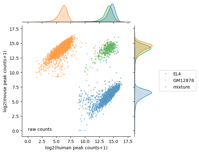
[12]:
plt.figure(figsize=(2, 2), dpi=150)

ax = sns.jointplot(data=raw_counts_df,
                   x="log2(human peak counts+1)",
                   y="log2(mouse peak counts+1)",
                   hue='species',
                   hue_order=['EL4', 'GM12878', 'mixture'],
                   s=8,
                   alpha=0.5,
                   legend=True,
                   height=5,
                   rasterized=True,
                   marginal_kws={'common_norm':False});
ax.ax_joint.text(0, 0, 'raw counts');

ax.ax_joint.set_xlim(-1, 18);
ax.ax_joint.set_ylim(-1, 18);
ax.ax_joint.legend(bbox_to_anchor=(1.6, 0.6),borderaxespad=0)
[12]:
<matplotlib.legend.Legend at 0x7f18698d5d00>
<Figure size 300x300 with 0 Axes>
[13]:
hgmm10k_scATACseq.obs['species'] = raw_counts_df['species']
Run scar#
[14]:
sc.pp.filter_genes(hgmm10k_scATACseq, min_counts=3000);
sc.pp.filter_genes(hgmm10k_scATACseq, max_counts=6500);
sc.pp.filter_cells(hgmm10k_scATACseq, min_genes=1700);
[15]:
setup_anndata(
    adata = hgmm10k_scATACseq,
    raw_adata = hgmm10k_scATACseq_raw,
    prob = 0.998,
    kneeplot = True
)
2024-08-10 21:12:34|INFO|setup_anndata|Use all 234078 droplets.
2024-08-10 21:12:34|INFO|setup_anndata|Estimating ambient profile for ['Peaks']...
2024-08-10 21:13:06|INFO|setup_anndata|Iteration: 1
2024-08-10 21:13:37|INFO|setup_anndata|Iteration: 2
2024-08-10 21:14:09|INFO|setup_anndata|Iteration: 3
2024-08-10 21:14:09|INFO|setup_anndata|Estimated ambient profile for Peaks saved in adata.uns
2024-08-10 21:14:09|INFO|setup_anndata|Estimated ambient profile for all features saved in adata.uns

[16]:
hgmm10k_scATACseq.uns['ambient_profile_Peaks']
[16]:
| ambient_profile_Peaks | |
|---|---|
| GRCh38_chr1:778276-779184 | 0.000034 |
| GRCh38_chr1:958857-959725 | 0.000034 |
| GRCh38_chr1:1012966-1013877 | 0.000022 |
| GRCh38_chr1:1019134-1020005 | 0.000101 |
| GRCh38_chr1:1032743-1033658 | 0.000028 |
| ... | ... |
| mm10_chrX:166479303-166480165 | 0.000073 |
| mm10_chrX:167382297-167383097 | 0.000056 |
| mm10_chrX:169986707-169987568 | 0.000034 |
| mm10_chrY:90741457-90742113 | 0.000062 |
| mm10_JH584304.1:26551-27398 | 0.000090 |
16080 rows × 1 columns
[17]:
raw_counts = hgmm10k_scATACseq.to_df()
raw_counts.head()
[17]:
| GRCh38_chr1:778276-779184 | GRCh38_chr1:958857-959725 | GRCh38_chr1:1012966-1013877 | GRCh38_chr1:1019134-1020005 | GRCh38_chr1:1032743-1033658 | GRCh38_chr1:1059198-1060047 | GRCh38_chr1:1063769-1064659 | GRCh38_chr1:1231630-1232529 | GRCh38_chr1:1273493-1274386 | GRCh38_chr1:1324324-1325228 | ... | mm10_chrX:163549410-163550287 | mm10_chrX:163879142-163880015 | mm10_chrX:163958369-163958813 | mm10_chrX:164381674-164382588 | mm10_chrX:166440266-166441175 | mm10_chrX:166479303-166480165 | mm10_chrX:167382297-167383097 | mm10_chrX:169986707-169987568 | mm10_chrY:90741457-90742113 | mm10_JH584304.1:26551-27398 | |
|---|---|---|---|---|---|---|---|---|---|---|---|---|---|---|---|---|---|---|---|---|---|
| AAACGAAAGATGTTCC-1 | 0.0 | 0.0 | 0.0 | 2.0 | 0.0 | 0.0 | 0.0 | 0.0 | 0.0 | 0.0 | ... | 0.0 | 0.0 | 0.0 | 0.0 | 0.0 | 0.0 | 0.0 | 0.0 | 0.0 | 0.0 |
| AAACGAAAGCTTACCA-1 | 0.0 | 2.0 | 0.0 | 0.0 | 0.0 | 2.0 | 0.0 | 0.0 | 2.0 | 2.0 | ... | 0.0 | 0.0 | 0.0 | 0.0 | 0.0 | 0.0 | 0.0 | 0.0 | 0.0 | 0.0 |
| AAACGAACAACTCGTA-1 | 0.0 | 4.0 | 0.0 | 2.0 | 0.0 | 0.0 | 0.0 | 7.0 | 0.0 | 4.0 | ... | 0.0 | 0.0 | 0.0 | 0.0 | 0.0 | 0.0 | 0.0 | 0.0 | 0.0 | 0.0 |
| AAACGAACACAGAAGC-1 | 0.0 | 0.0 | 12.0 | 2.0 | 0.0 | 0.0 | 0.0 | 0.0 | 0.0 | 0.0 | ... | 0.0 | 0.0 | 0.0 | 0.0 | 0.0 | 0.0 | 0.0 | 0.0 | 0.0 | 0.0 |
| AAACGAACATAAAGTG-1 | 4.0 | 0.0 | 2.0 | 4.0 | 0.0 | 0.0 | 0.0 | 0.0 | 0.0 | 0.0 | ... | 0.0 | 0.0 | 0.0 | 0.0 | 0.0 | 0.0 | 0.0 | 0.0 | 0.0 | 0.0 |
5 rows × 16080 columns
[18]:
ambient_profile = hgmm10k_scATACseq.uns["ambient_profile_Peaks"]
ambient_profile.head()
[18]:
| ambient_profile_Peaks | |
|---|---|
| GRCh38_chr1:778276-779184 | 0.000034 |
| GRCh38_chr1:958857-959725 | 0.000034 |
| GRCh38_chr1:1012966-1013877 | 0.000022 |
| GRCh38_chr1:1019134-1020005 | 0.000101 |
| GRCh38_chr1:1032743-1033658 | 0.000028 |
[19]:
hgmm_10k_ATAC_scar = model(raw_count = raw_counts,
                           ambient_profile = ambient_profile, # In the case of default None, the ambient_profile will be calculated by averaging pooled cells
                           feature_type='ATAC',
                           sparsity=1,
                           device='cuda'
                          )

hgmm_10k_ATAC_scar.train(epochs=500,
                         batch_size=64,
                         verbose=True
                        )

# After training, we can infer the native true signal
hgmm_10k_ATAC_scar.inference()  # by defaut, batch_size = None, set a batch_size if getting a GPU memory issue
2024-08-10 21:14:13|INFO|model|cuda will be used.
2024-08-10 21:14:15|INFO|VAE|Running VAE using the following param set:
2024-08-10 21:14:15|INFO|VAE|...denoised count type: ATAC
2024-08-10 21:14:15|INFO|VAE|...count model: binomial
2024-08-10 21:14:15|INFO|VAE|...num_input_feature: 16080
2024-08-10 21:14:15|INFO|VAE|...NN_layer1: 150
2024-08-10 21:14:15|INFO|VAE|...NN_layer2: 100
2024-08-10 21:14:15|INFO|VAE|...latent_space: 15
2024-08-10 21:14:15|INFO|VAE|...dropout_prob: 0.00
2024-08-10 21:14:15|INFO|VAE|...expected data sparsity: 1.00
2024-08-10 21:14:15|INFO|model|kld_weight: 1.00e-05
2024-08-10 21:14:15|INFO|model|learning rate: 1.00e-03
2024-08-10 21:14:15|INFO|model|lr_step_size: 5
2024-08-10 21:14:15|INFO|model|lr_gamma: 0.97
Training: 100%|██████████| 500/500 [06:38<00:00, 1.25it/s, Loss=1.2114e+04]
[20]:
# The denoised counts are saved in scarObj.native_counts
denoised_counts = pd.DataFrame(hgmm_10k_ATAC_scar.native_counts.toarray(), index=raw_counts.index, columns=raw_counts.columns)
hgmm10k_scATACseq.layers['denoised_peaks_scAR'] = denoised_counts
[21]:
denoised_peaks_scAR = count_peaks(denoised_counts)
denoised_peaks_scAR['species'] = hgmm10k_scATACseq.obs['species']
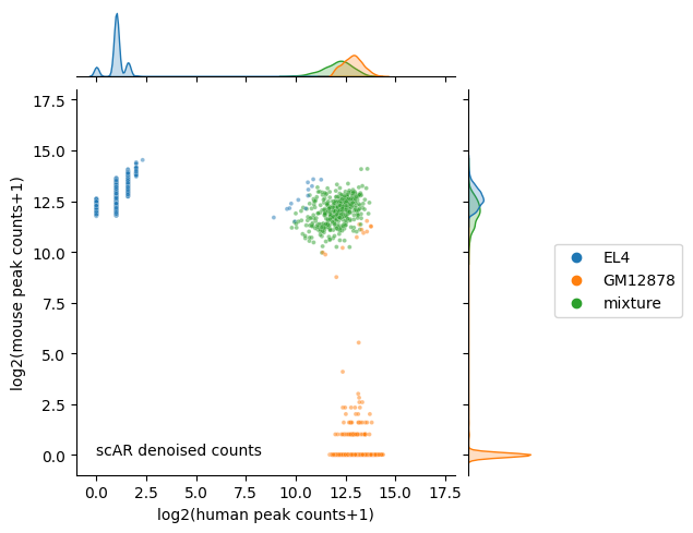
[22]:
plt.figure(figsize=(2, 2), dpi=150)

ax = sns.jointplot(data=denoised_peaks_scAR,
                   x="log2(human peak counts+1)",
                   y="log2(mouse peak counts+1)",
                   hue='species',
                   hue_order=['EL4', 'GM12878', 'mixture'],
                   s=8,
                   alpha=0.5,
                   legend=True,
                   height=5,
                   rasterized=True,
                   marginal_kws={'common_norm':False});
ax.ax_joint.text(0, 0, 'scAR denoised counts');

ax.ax_joint.set_xlim(-1, 18);
ax.ax_joint.set_ylim(-1, 18);
ax.ax_joint.legend(bbox_to_anchor=(1.6, 0.6),borderaxespad=0)
[22]:
<matplotlib.legend.Legend at 0x7f1869be1a30>
<Figure size 300x300 with 0 Axes>